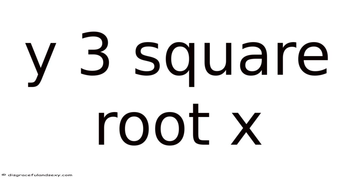
Unraveling the Mystery of y = 3∛x: A Comprehensive Exploration
The equation y = 3∛x might seem simple at first glance, but it embodies a rich tapestry of mathematical concepts, connecting algebra, geometry, and even calculus. This article delves deep into this seemingly uncomplicated equation, exploring its properties, graphical representation, transformations, and applications, making it accessible to a wide range of readers, from high school students to those brushing up on their math skills. Understanding this equation provides a solid foundation for tackling more complex mathematical problems involving radicals and functions Small thing, real impact..
I. Understanding the Basics: Cubes and Cube Roots
Before we embark on a detailed analysis of y = 3∛x, let's solidify our understanding of the fundamental building blocks: cubes and cube roots.
A cube of a number is the result of multiplying that number by itself three times. To give you an idea, the cube of 2 (written as 2³) is 2 * 2 * 2 = 8. Similarly, the cube of 5 (5³) is 5 * 5 * 5 = 125 That's the whole idea..
The cube root, denoted by the symbol ∛, is the inverse operation of cubing. It answers the question, "What number, when multiplied by itself three times, gives the given number?" Here's one way to look at it: the cube root of 8 (∛8) is 2, because 2 * 2 * 2 = 8. Similarly, ∛125 = 5.
In our equation, y = 3∛x, we see the cube root of x multiplied by 3. Basically, the output y is three times the cube root of the input x.
II. Graphing the Function: Visualizing y = 3∛x
Visualizing the function is crucial for understanding its behavior. The graph of y = 3∛x is a transformation of the basic cube root function, y = ∛x But it adds up..
-
The Parent Function (y = ∛x): The graph of y = ∛x passes through the origin (0,0) and increases steadily as x increases. It's a smooth curve that extends infinitely in both the positive and negative x and y directions. you'll want to note that the cube root function is defined for all real numbers, including negative numbers. Take this: ∛-8 = -2.
-
Transformation: y = 3∛x: The '3' in our equation acts as a vertical stretch. It stretches the graph of y = ∛x vertically by a factor of 3. What this tells us is for any given x, the corresponding y value will be three times larger than in the parent function. The graph will still pass through the origin (0,0) but will rise more steeply than y = ∛x.
III. Key Properties of y = 3∛x
Let's break down the key properties that characterize the function y = 3∛x:
-
Domain: The domain of a function represents all possible input values (x) for which the function is defined. Since we can take the cube root of any real number (positive, negative, or zero), the domain of y = 3∛x is all real numbers, denoted as (-∞, ∞) And that's really what it comes down to..
-
Range: The range of a function is the set of all possible output values (y). Because the cube root function can produce any real number, and we are multiplying it by 3, the range of y = 3∛x is also all real numbers, (-∞, ∞) Practical, not theoretical..
-
x-intercept and y-intercept: The x-intercept is the point where the graph intersects the x-axis (where y = 0). Setting y = 0 in our equation, we get 0 = 3∛x, which implies ∛x = 0, and thus x = 0. The x-intercept is (0, 0). Similarly, the y-intercept is also (0, 0) since when x = 0, y = 0.
-
Increasing/Decreasing: The function y = 3∛x is strictly increasing. As x increases, y also increases. This is a characteristic of cube root functions.
-
Continuity: The function is continuous; there are no breaks or jumps in the graph. It's a smooth, unbroken curve.
-
Symmetry: The function is not symmetrical about the y-axis (even function) nor the origin (odd function).
IV. Applications of y = 3∛x
While seemingly abstract, the function y = 3∛x and its variations have real-world applications:
-
Modeling Growth: Cube root functions can model certain types of growth processes where the rate of growth slows down over time. Here's a good example: it might be used to model the growth of a certain type of plant or the spread of a particular disease under specific conditions. The factor of 3 would simply scale the growth rate Small thing, real impact..
-
Engineering and Physics: Cube root functions appear in various physics and engineering problems. As an example, they can be used in calculating the relationship between the volume and the side length of a cube Small thing, real impact..
-
Data Analysis: In data analysis, cube root transformations are sometimes used to stabilize variance in a dataset or to make the data more normally distributed, which can improve the accuracy of statistical models But it adds up..
-
Economics: While less directly apparent, variations of cube root functions can appear in certain economic models that involve diminishing returns or other non-linear relationships.
V. Transformations and Variations
Understanding the basic function y = 3∛x allows us to predict the behavior of related functions through transformations:
-
Vertical Shifts: Adding a constant to the function, such as y = 3∛x + 2, shifts the graph vertically upwards by 2 units. Subtracting a constant shifts it downwards Not complicated — just consistent..
-
Horizontal Shifts: The function y = 3∛(x - 1) shifts the graph horizontally to the right by 1 unit. Adding a constant inside the cube root shifts it to the left.
-
Vertical Stretches/Compressions: Multiplying the function by a constant other than 3, like y = 2∛x or y = 5∛x, changes the steepness of the curve. Values greater than 3 will result in a steeper curve, while values between 0 and 3 will make it less steep.
-
Reflections: Adding a negative sign in front of the function, y = -3∛x, reflects the graph across the x-axis. A negative sign inside the cube root, y = 3∛(-x), reflects the graph across the y-axis.
VI. Calculus and the Cube Root Function
For those familiar with calculus, let's examine the derivative and integral of y = 3∛x:
-
Derivative: The derivative of y = 3∛x (which can be written as y = 3x^(1/3)) is found using the power rule: dy/dx = 3 * (1/3) * x^(-2/3) = x^(-2/3) = 1/x^(2/3). This derivative is undefined at x = 0, reflecting the vertical tangent at that point on the graph Worth knowing..
-
Integral: The indefinite integral of y = 3∛x is found using the power rule for integration: ∫3x^(1/3) dx = 3 * (3/4) * x^(4/3) + C = (9/4)x^(4/3) + C, where C is the constant of integration That's the part that actually makes a difference..
VII. Frequently Asked Questions (FAQ)
Q: What is the difference between y = ∛x and y = 3∛x?
A: y = ∛x is the basic cube root function. y = 3∛x is a vertical stretch of this function by a factor of 3. Every y-value in y = 3∛x is three times the corresponding y-value in y = ∛x Simple, but easy to overlook..
Q: Can I have a negative value for x in y = 3∛x?
A: Yes, the cube root of a negative number is a real number. Also, for example, ∛(-8) = -2. That's why, you can input any real number for x Simple as that..
Q: What is the inverse function of y = 3∛x?
A: To find the inverse function, we switch x and y and solve for y: x = 3∛y. Dividing by 3, we get x/3 = ∛y. Cubing both sides gives us y = (x/3)³. So, the inverse function is y = (x/3)³.
Honestly, this part trips people up more than it should That's the part that actually makes a difference..
Q: How do I solve equations involving y = 3∛x?
A: Solving equations involving this function usually requires isolating the cube root term and then cubing both sides to eliminate the radical. As an example, if you have the equation 5 = 3∛x, you would divide by 3 to get 5/3 = ∛x, and then cube both sides: (5/3)³ = x The details matter here..
VIII. Conclusion
The seemingly simple equation y = 3∛x reveals a fascinating interplay of mathematical concepts. That said, by understanding its graphical representation, properties, transformations, and applications, we gain a deeper appreciation of the power and versatility of mathematical functions. This exploration goes beyond rote memorization; it fosters a deeper understanding of how mathematical concepts connect and interact, enriching your mathematical journey and equipping you with the tools to tackle more complex problems in the future. This function, while seemingly elementary, serves as a dependable stepping stone to understanding more complex mathematical ideas.
